Understanding RBMs

Restricted Boltzmann machines are at the heart of many deep-learning nets as well as neural nets’ renaissance, so their mechanism deserves a bit more attention.

To walk through the process of how an RBM works, we’ll use the example of MNIST, a collection of images representing the handwritten numerals zero through nine, which RBMs are typically trained to recognize and classify in order to prove that they function at all.

Each RBM has just two “node” layers, a visible layer and a hidden one. The first, visible, layer receives input; that is, the data you feed into the net to be learned. You can think of the RBM’s input nodes as receptacles into which random samples of data are placed. They’re boxes, each holding a data point, which in the initial layer would be a sampling of pixels.

To the RBM, each image is nothing more than a collection of pixels that it must classify. The only way to classify images is by their features, the distinctive characteristics of the pixels. Those are generally dark hues and light ones lined up along edges, curves, corners, peaks and intersections — the stuff that handwritten numerals and their backgrounds are made of, their constituent parts.

As it iterates over MNIST, an RBM is fed one numeral-image at a time without knowing what it is. In a sense, the RBM is behind a veil of ignorance, and its entire purpose is to learn what numeral it is dealing with behind the veil by randomly sampling pixels from the numeral’s unseen image, and testing which ones lead it to correctly identify the number. (There is a benchmark dataset, the test set, that knows the answers, and against which the RBM-in-training contrasts its own, provisional conclusions.)

Each time the RBM guesses wrong, it is told to go back and try again, until it discovers the pixels that best indicate the numeral they’re a part of – the signals that improve its capacity to classify. The connections among nodes that led it to the wrong conclusion are punished, or discounted. They grow weaker as the net searches for a path toward greater accuracy and less error.

Invisible Cities

Since it’s a stretch to even imagine an entity that cannot identify numbers, one way to explain how RBMs work is through analogy.

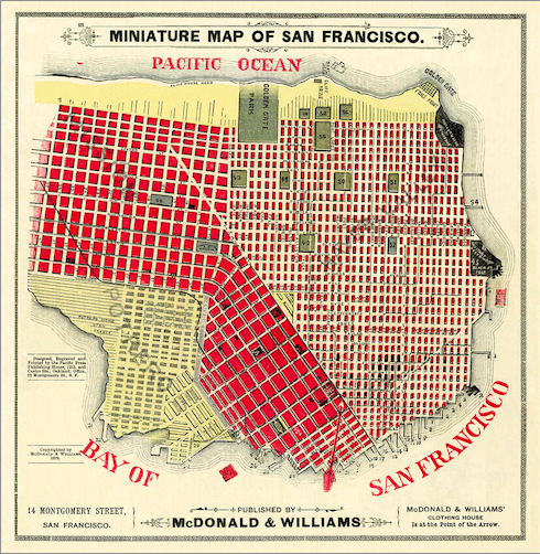
Imagine each numeral-image like an invisible city, one of ten whose names you know: San Francisco, New York, New Orleans, Seattle… An RBM starts by reaching into the invisible city, touching various points on its streets and crossings. If it brought back a “Washington St.,” one of the most common street names in America, it would know little about the city it sought to identify. This would be akin to sampling an image and bringing back pixels from its black background, rather than an edge that formed one of the numeral’s lines or kinks. The backdrop tells you almost nothing useful of the data structure you must classify. Those indistinguishable pixels are Washington St.

Let’s take Market St instead… New York, New Orleans, Seattle and San Francisco all have Market Streets of different lengths and orientations. An invisible city that returns many samples labeled Market Street is more likely to be San Francisco or Seattle, which have longer Market Streets, than New York or New Orleans.

By analogy, 2s, 3s, 5s, 6s, 8s and 9s all have curves, but an unknown numeral-image with a curve as a feature is less likely to be a 1, 4 or 7. So an RBM, with time, will learn that curves are decent indicators of some numbers and not others. They will learn to weight the path connecting the curve node to a 2 or 3 label more heavily than the path extending toward a 1 or 4.

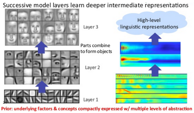
In fact, the process is slightly more complex, because RBMs can be stacked to gradually aggregate groups of features, layer upon layer. These stacks are called deep-belief nets, and deep-belief nets are valuable because each RBM within them deals with more and more complex ensembles of features until they group enough together to recognize the whole: pixel (input), line, chin, jaw, lower face, visage, name of person (label).

But let’s stick with the city and take just two features together. If an urban data sample shows an intersection of Market and an avenue named Van Ness, then the likelihood that it is San Francisco is high. Likewise, if data samples from the numeral-image show a vertical bar meeting a partial circle that opens to the left, then we very likely have a 5 and nothing else.

Now let’s imagine both the numeral-images and invisible cities as maps whose points are connected to each other as probabilities. If you start from a curve on an 8 (even if you don’t know it’s an 8), the probability of landing on another curve at some point is nearly 100%; if you are on a five, that probability is lower.

Likewise, if you start from Market in San Francisco, even if you don’t know you are in San Francisco, you have a high probability of hitting Van Ness at some point, given that the two streets bisect the city and cross each other at the center.

The simple feature of hitting Market Street (which is on an early hidden layer of the deep-belief net) leads to another feature, both more complex and more rare, of hitting both Market and Van Ness, which would be represented on a later node layer aggregating the two features.

But maybe you are not in San Francisco at all. Market and Van Ness is not the only node as you move deeper in.

The hidden nodes in subsequent layers of the DBN should allow for states (data conditions) that could only occur in other cities: e.g. the combination of Market and FDR Drive places you with high probability in New York; the combination of Market with Shilshole avenue in Seattle. (Likewise, starting from a curve feature at the input node, you could end up intersecting with a vertical bar indicating a 5, or with another curve pointing you toward an 8.)

So maybe from your initial Market Street data point, you would have a 50 percent chance of ending up with Van Ness as well; a 10 percent chance of getting FDR; and a 20 percent chance of Shilshole. But from the deeper node of Market + Van Ness, you have a 99 percent chance of ending up classified as San Francisco. The same goes for New York and Seattle, respectively.

Likewise, while many numeral-images — 1, 4, 5 and 7 — contain more or less vertical bars, only three of them also contain horizontal bars. And of those, only the 4 allows the two bars to cross forming four 90 degree angles. Thus, enlarging the groups of features per node as you move deeper also raises the likelihood that those increasingly rare feature-groups correlate with a single numeral-image.

Markov Chains

RBMs tie all their nodes together in an algorithm called a Markov Chain. Markov Chains are essentially logical circuits that connect two or more states via probabilities. A sequence of coin flips, a series of die rolls, Rozencrantz and Guildenstern marching toward their fate.

Let’s explore this idea with another absurdly long analogy.

We’ll imagine a universe where you have three possible locations, or states, which we’ll call home, office and bowling alley. Those three states are linked by probabilities, which represent the likelihood that you’ll move from one to the other.

At any given moment when you’re home, there is a low probability of you going to the bowling alley, let’s say 10%, a midsize one of going to the office, 40%, and a high one of you remaining where you are, let’s say 50%. The probabilities exiting any one state should always add up to 100%.

Now let’s take the bowling alley: At any given moment while you’re there, there’s a low probability of you remaining amid the beer and slippery shoes, since people don’t bowl for more than a few hours, a low one of going to the office, since work tends to come before bowling, and a high one of you returning home. Let’s make those 20%, 10% and 70%.

So a home state is a fair indication of office state, and a poor indication of bowling alley state. While bowling alley state is a great indicator of home state and a poor indicator of office state. (We’re skipping office state because you get the point.) Each state is in a garden of forking paths, but the paths are not equal.

Markov Chains are sequential. Their purpose is to give you a good idea, given one state, of what the next one will be. Instead of home, office and bowling alley, those states might be edge, intersection and numeral-image, or street, neighborhood and city. Markov Chains are also good for predicting which word is most likely to follow a given wordset (useful in natural-language processing), or which share price is likely to follow a given sequence of share prices (useful in making lots of money).

Remember that RBMs are being tested for accuracy against a benchmark dataset, and they record the features that lead them to the correct conclusion. Their job is to learn and adjust the probabilities between the feature-nodes in such a way that if the RBM receives a certain feature, which is a strong indicator of a 5, then the probabilities between nodes lead it to conclude it’s in the presence of a 5. They register which features, feature groups and numeral-images tend to light up together.

Now, if you’re ready, we’ll show you how to implement a deep-belief network.