A Beginner’s Guide to Recurrent Networks and LSTMs
Contents
- Feedforward Networks
- Recurrent Networks
- Backpropagation Through Time
- Vanishing and Exploding Gradients
- Long Short-Term Memory Units (LSTMs)
- Capturing Diverse Time Scales
- Code Sample & Comments
- Resources
The purpose of this post is to give students of neural networks an intuition about the functioning of recurrent neural networks and purpose and structure of a prominent RNN variation, LSTMs.
Recurrent nets are a type of artificial neural network designed to recognize patterns in sequences of data, such as text, genomes, handwriting, the spoken word, or numerical times series data emanating from sensors, stock markets and government agencies.
They are arguably the most powerful and useful type of neural network, applicable even to images, which can be decomposed into a series of patches and treated as a sequence.
Since recurrent networks possess a certain type of memory, and memory is also part of the human condition, we’ll make repeated analogies to memory in the brain.1
Review of Feedforward Networks
To understand recurrent nets, first you have to understand the basics of feedforward nets. Both of these networks are named after the way they channel information through a series of mathematical operations performed at the nodes of the network. One feeds information straight through (never touching a given node twice), while the other cycles it through a loop, and the latter are called recurrent.
In the case of feedforward networks, input examples are fed to the network and transformed into an output; with supervised learning, the output would be a label, a name applied to the input. That is, they map raw data to categories, recognizing patterns that may signal, for example, that an input image should be labeled “cat” or “elephant.”
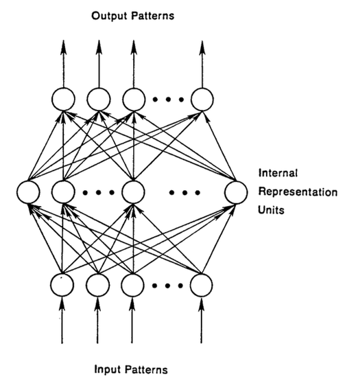
A feedforward network is trained on labeled images until it minimizes the error it makes when guessing their categories. With the trained set of parameters (or weights, collectively known as a model), the network sallies forth to categorize data it has never seen. A trained feedforward network can be exposed to any random collection of photographs, and the first photograph it is exposed to will not necessarily alter how it classifies the second. Seeing photograph of a cat will not lead the net to perceive an elephant next.
That is, a feedforward network has no notion of order in time, and the only input it considers is the current example it has been exposed to. Feedforward networks are amnesiacs regarding their recent past; they remember nostalgically only the formative moments of training.
Recurrent Networks
Recurrent networks, on the other hand, take as their input not just the current input example they see, but also what they have perceived previously in time. Here’s a diagram of an early, simple recurrent net proposed by Elman, where the BTSXPE at the bottom of the drawing represents the input example in the current moment, and CONTEXT UNIT represents the output of the previous moment.
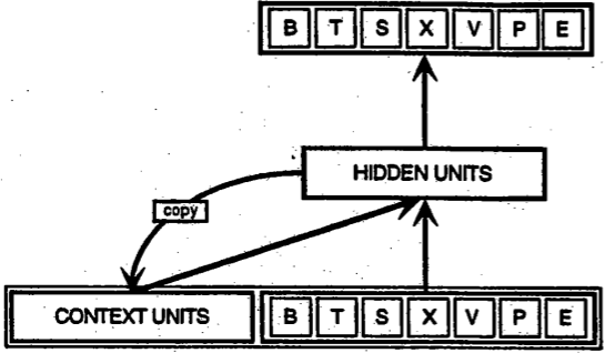
The decision a recurrent net reached at time step t-1 affects the decision it will reach one moment later at time step t. So recurrent networks have two sources of input, the present and the recent past, which combine to determine how they respond to new data, much as we do in life.
Recurrent networks are distinguished from feedforward networks by that feedback loop connected to their past decisions, ingesting their own outputs moment after moment as input. It is often said that recurrent networks have memory.2 Adding memory to neural networks has a purpose: There is information in the sequence itself, and recurrent nets use it to perform tasks that feedforward networks can’t.
That sequential information is preserved in the recurrent network’s hidden state, which manages to span many time steps as it cascades forward to affect the processing of each new example. It is finding correlations between events separated by many moments, and these correlations are called “long-term dependencies”, because an event downstream in time depends upon, and is a function of, one or more events that came before. One way to think about RNNs is this: they are a way to share weights over time.
Just as human memory circulates invisibly within a body, affecting our behavior without revealing its full shape, information circulates in the hidden states of recurrent nets. The English language is full of words that describe the feedback loops of memory. When we say a person is haunted by their deeds, for example, we are simply talking about the consequences that past outputs wreak on present time. The French call this “Le passé qui ne passe pas,” or “The past that does not pass away.”
We’ll describe the process of carrying memory forward mathematically:

The hidden state at time step t is h_t. It is a function of the input at the same time step x_t, modified by a weight matrix W (like the one we used for feedforward nets) added to the hidden state of the previous time step h_t-1 multiplied by its own hidden-state-to-hidden-state matrix U, otherwise known as a transition matrix and similar to a Markov chain. The weight matrices are filters that determine how much importance to accord to both the present input and the past hidden state. The error they generate will return via backpropagation and be used to adjust their weights until error can’t go any lower.
The sum of the weight input and hidden state is squashed by the function φ – either a logistic sigmoid function or tanh, depending – which is a standard tool for condensing very large or very small values into a logistic space, as well as making gradients workable for backpropagation.
Because this feedback loop occurs at every time step in the series, each hidden state contains traces not only of the previous hidden state, but also of all those that preceded h_t-1 for as long as memory can persist.
Given a series of letters, a recurrent will use the first character to help determine its perception of the second character, such that an initial q might lead it to infer that the next letter will be u, while an initial t might lead it to infer that the next letter will be h.
Since recurrent nets span time, they are probably best illustrated with animation (the first vertical line of nodes to appear can be thought of as a feedforward network, which becomes recurrent as it unfurls over time).
how recurrent neural networks work #deeplearning4j #dl4j
In the diagram above, each x is an input example, w is the weights that filter inputs, a is the activation of the hidden layer (a combination of weighted input and the previous hidden state), and b is the output of the hidden layer after it has been transformed, or squashed, using a rectified linear or sigmoid unit.
Backpropagation Through Time (BPTT)
Remember, the purpose of recurrent nets is to accurately classify sequential input. We rely on the backpropagation of error and gradient descent to do so.
Backpropagation in feedforward networks moves backward from the final error through the outputs, weights and inputs of each hidden layer, assigning those weights responsibility for a portion of the error by calculating their partial derivatives – ∂E/∂w, or the relationship between their rates of change. Those derivatives are then used by our learning rule, gradient descent, to adjust the weights up or down, whichever direction decreases error.
Recurrent networks rely on an extension of backpropagation called backpropagation through time, or BPTT. Time, in this case, is simply expressed by a well-defined, ordered series of calculations linking one time step to the next, which is all backpropagation needs to work.
Neural networks, whether they are recurrent or not, are simply nested composite functions like f(g(h(x))). Adding a time element only extends the series of functions for which we calculate derivatives with the chain rule.
Truncated BPTT
Truncated BPTT is an approximation of full BPTT that is preferred for long sequences, since full BPTT’s forward/backward cost per parameter update becomes very high over many time steps. The downside is that the gradient can only flow back so far due to that truncation, so the network can’t learn dependencies that are as long as in full BPTT.
Vanishing (and Exploding) Gradients
Like most neural networks, recurrent nets are old. By the early 1990s, the vanishing gradient problem emerged as a major obstacle to recurrent net performance.
Just as a straight line expresses a change in x alongside a change in y, the gradient expresses the change in all weights with regard to the change in error. If we can’t know the gradient, we can’t adjust the weights in a direction that will decrease error, and our network ceases to learn.
Recurrent nets seeking to establish connections between a final output and events many time steps before were hobbled, because it is very difficult to know how much importance to accord to remote inputs. (Like great-great-*-grandparents, they multiply quickly in number and their legacy is often obscure.)
This is partially because the information flowing through neural nets passes through many stages of multiplication.
Everyone who has studied compound interest knows that any quantity multiplied frequently by an amount slightly greater than one can become immeasurably large (indeed, that simple mathematical truth underpins network effects and inevitable social inequalities). But its inverse, multiplying by a quantity less than one, is also true. Gamblers go bankrupt fast when they win just 97 cents on every dollar they put in the slots.
Because the layers and time steps of deep neural networks relate to each other through multiplication, derivatives are susceptible to vanishing or exploding.
Exploding gradients treat every weight as though it were the proverbial butterfly whose flapping wings cause a distant hurricane. Those weights’ gradients become saturated on the high end; i.e. they are presumed to be too powerful. But exploding gradients can be solved relatively easily, because they can be truncated or squashed. Vanishing gradients can become too small for computers to work with or for networks to learn – a harder problem to solve.
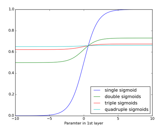
Below you see the effects of applying a sigmoid function over and over again. The data is flattened until, for large stretches, it has no detectable slope. This is analogous to a gradient vanishing as it passes through many layers.
Long Short-Term Memory Units (LSTMs)
In the mid-90s, a variation of recurrent net with so-called Long Short-Term Memory units, or LSTMs, was proposed by the German researchers Sepp Hochreiter and Juergen Schmidhuber as a solution to the vanishing gradient problem.
LSTMs help preserve the error that can be backpropagated through time and layers. By maintaining a more constant error, they allow recurrent nets to continue to learn over many time steps (over 1000), thereby opening a channel to link causes and effects remotely. This is one of the central challenges to machine learning and AI, since algorithms are frequently confronted by environments where reward signals are sparse and delayed, such as life itself. (Religious thinkers have tackled this same problem with ideas of karma or divine reward, theorizing invisible and distant consequences to our actions.)
LSTMs contain information outside the normal flow of the recurrent network in a gated cell. Information can be stored in, written to, or read from a cell, much like data in a computer’s memory. The cell makes decisions about what to store, and when to allow reads, writes and erasures, via gates that open and close. Unlike the digital storage on computers, however, these gates are analog, implemented with element-wise multiplication by sigmoids, which are all in the range of 0-1. Analog has the advantage over digital of being differentiable, and therefore suitable for backpropagation.
Those gates act on the signals they receive, and similar to the neural network’s nodes, they block or pass on information based on its strength and import, which they filter with their own sets of weights. Those weights, like the weights that modulate input and hidden states, are adjusted via the recurrent networks learning process. That is, the cells learn when to allow data to enter, leave or be deleted through the iterative process of making guesses, backpropagating error, and adjusting weights via gradient descent.
The diagram below illustrates how data flows through a memory cell and is controlled by its gates.
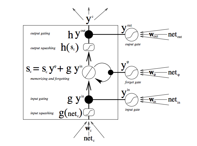
There are a lot of moving parts here, so if you are new to LSTMs, don’t rush this diagram – contemplate it. After a few minutes, it will begin to reveal its secrets.
Starting from the bottom, the triple arrows show where information flows into the cell at multiple points. That combination of present input and past cell state is fed not only to the cell itself, but also to each of its three gates, which will decide how the input will be handled.
The black dots are the gates themselves, which determine respectively whether to let new input in, erase the present cell state, and/or let that state impact the network’s output at the present time step. S_c is the current state of the memory cell, and g_y_in is the current input to it. Remember that each gate can be open or shut, and they will recombine their open and shut states at each step. The cell can forget its state, or not; be written to, or not; and be read from, or not, at each time step, and those flows are represented here.
The large bold letters give us the result of each operation.
Here’s another diagram for good measure, comparing a simple recurrent network (left) to an LSTM cell (right). The blue lines can be ignored; the legend is helpful.
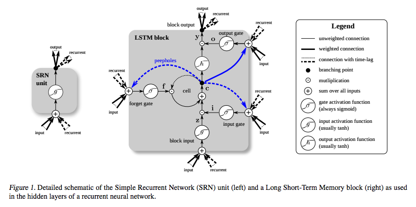
It’s important to note that LSTMs’ memory cells give different roles to addition and multiplication in the transformation of input. The central plus sign in both diagrams is essentially the secret of LSTMs. Stupidly simple as it may seem, this basic change helps them preserve a constant error when it must be backpropagated at depth. Instead of determining the subsequent cell state by multiplying its current state with new input, they add the two, and that quite literally makes the difference. (The forget gate still relies on multiplication, of course.)
Different sets of weights filter the input for input, output and forgetting. The forget gate is represented as a linear identity function, because if the gate is open, the current state of the memory cell is simply multiplied by one, to propagate forward one more time step.
Furthermore, while we’re on the topic of simple hacks, including a bias of 1 to the forget gate of every LSTM cell is also shown to improve performance. (Sutskever, on the other hand, recommends a bias of 5.)
You may wonder why LSTMs have a forget gate when their purpose is to link distant occurrences to a final output. Well, sometimes it’s good to forget. If you’re analyzing a text corpus and come to the end of a document, for example, you may have no reason to believe that the next document has any relationship to it whatsoever, and therefore the memory cell should be set to zero before the net ingests the first element of the next document.
In the diagram below, you can see the gates at work, with straight lines representing closed gates, and blank circles representing open ones. The lines and circles running horizontal down the hidden layer are the forget gates.
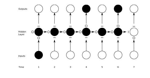
It should be noted that while feedforward networks map one input to one output, recurrent nets can map one to many, as above (one image to many words in a caption), many to many (translation), or many to one (classifying a voice).
Capturing Diverse Time Scales and Remote Dependencies
You may also wonder what the precise value is of input gates that protect a memory cell from new data coming in, and output gates that prevent it from affecting certain outputs of the RNN. You can think of LSTMs as allowing a neural network to operate on different scales of time at once.
Let’s take a human life, and imagine that we are receiving various streams of data about that life in a time series. Geolocation at each time step is pretty important for the next time step, so that scale of time is always open to the latest information.
Perhaps this human is a diligent citizen who votes every couple years. On democratic time, we would want to pay special attention to what they do around elections, before they return to making a living, and away from larger issues. We would not want to let the constant noise of geolocation affect our political analysis.
If this human is also a diligent daughter, then maybe we can construct a familial time that learns patterns in phone calls which take place regularly every Sunday and spike annually around the holidays. Little to do with political cycles or geolocation.
Other data is like that. Music is polyrhythmic. Text contains recurrent themes at varying intervals. Stock markets and economies experience jitters within longer waves. They operate simultaneously on different time scales that LSTMs can capture.
Gated Recurrent Units (GRUs)
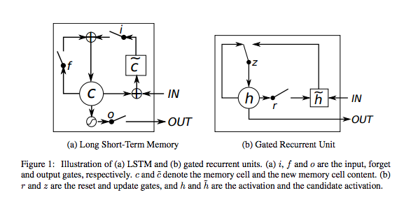
A gated recurrent unit (GRU) is basically an LSTM without an output gate, which therefore fully writes the contents from its memory cell to the larger net at each time step.
Code Sample
A commented example of a Graves LSTM learning how to replicate Shakespearian drama, and implemented with Deeplearning4j, can be found here. The API is commented where it’s not self-explanatory. If you have questions, please join us on Gitter.
Here’s what the LSTM configuration looks like:
GET STARTED WITH DEEP LEARNING
LSTM Hyperparameter Tuning
Here are a few ideas to keep in mind when manually optimizing hyperparameters for RNNs:
- Watch out for overfitting, which happens when a neural network essentially “memorizes” the training data. Overfitting means you get great performance on training data, but the network’s model is useless for out-of-sample prediction.
- Regularization helps: regularization methods include l1, l2, and dropout among others.
- So have a separate test set on which the network doesn’t train.
- The larger the network, the more powerful, but it’s also easier to overfit. Don’t want to try to learn a million parameters from 10,000 examples –
parameters > examples = trouble. - More data is almost always better, because it helps fight overfitting.
- Train over multiple epochs (complete passes through the dataset).
- Evaluate test set performance at each epoch to know when to stop (early stopping).
- The learning rate is the single most important hyperparameter. Tune this using deeplearning4j-ui; see this graph
- In general, stacking layers can help.
- For LSTMs, use the softsign (not softmax) activation function over tanh (it’s faster and less prone to saturation (~0 gradients)).
- Updaters: RMSProp, AdaGrad or momentum (Nesterovs) are usually good choices. AdaGrad also decays the learning rate, which can help sometimes.
- Finally, remember data normalization, MSE loss function + identity activation function for regression, Xavier weight initialization
Resources
- DRAW: A Recurrent Neural Network For Image Generation; (attention models)
- Gated Feedback Recurrent Neural Networks
- Recurrent Neural Networks; Juergen Schmidhuber
- Modeling Sequences With RNNs and LSTMs; Geoff Hinton
- The Unreasonable Effectiveness of Recurrent Neural Networks; Andrej Karpathy
- Understanding LSTMs; Christopher Olah
- Backpropagation Through Time: What It Does and How to Do It; Paul Werbos
- Empirical Evaluation of Gated Recurrent Neural Networks on Sequence Modeling; Cho et al
- Training Recurrent Neural Networks; Ilya Sutskever’s Dissertation
- Supervised Sequence Labelling with Recurrent Neural Networks; Alex Graves
- Long Short-Term Memory in Recurrent Neural Networks; Felix Gers
- LSTM: A Search Space Oddyssey; Klaus Greff et al
More Machine Learning Tutorials
- Introduction to Neural Networks
- Beginner’s Guide to Reinforcement Learning
- Convolutional Networks (CNNs)
- Multilayer Perceptron (MLPs) for Classification
- Generative Adversarial Networks (GANs)
- Graph Data and Deep Learning
- Word2Vec: Neural Embeddings for NLP
- Symbolic Reasoning (Symbolic AI) & Deep Learning
- Markov Chain Monte Carlo & Machine Learning
- Restricted Boltzmann Machines
- Eigenvectors, Eigenvalues, Covariance, PCA and Entropy
- Neural Networks & Regression
- Introduction to Decision Trees
- Introduction to Random Forests
- Open Datasets for Machine Learning
- AI vs. Machine Learning vs. Deep Learning
- Inference in Production: Machine Learning Model Server
Footnotes
1) While recurrent networks may seem like a far cry from general artificial intelligence, it’s our belief that intelligence, in fact, is probably dumber than we thought. That is, with a simple feedback loop to serve as memory, we have one of the basic ingredients of consciousness – a necessary but insufficient component. Others, not discussed above, might include additional variables that represent the network and its state, and a framework for decisionmaking logic based on interpretations of data. The latter, ideally, would be part of a larger problem-solving loop that rewards success and punishes failure, much like reinforcement learning. Come to think of it, DeepMind already built that…
2) All neural networks whose parameters have been optimized have memory in a sense, because those parameters are the traces of past data. But in feedforward networks, that memory may be frozen in time. That is, after a network is trained, the model it learns may be applied to more data without further adapting itself. In addition, it is monolithic in the sense that the same memory (or set of weights) is applied to all incoming data. Recurrent networks, which also go by the name of dynamic (translation: “changing”) neural networks, are distinguished from feedforward nets not so much by having memory as by giving particular weight to events that occur in a series. While those events do not need to follow each other immediately, they are presumed to be linked, however remotely, by the same temporal thread. Feedforward nets do not make such a presumption. They treat the world as a bucket of objects without order or time. It may be helpful to map two types of neural network to two types of human knowledge. When we are children, we learn to recognize colors, and we go through the rest of our lives recognizing colors wherever we see them, in highly varied contexts and independent of time. We only had to learn the colors once. That knowledge is like memory in feedforward nets; they rely on a past without scope, undefined. Ask them what colors they were fed five minutes ago and they don’t know or care. They are short-term amnesiacs. On the other hand, we also learn as children to decipher the flow of sound called language, and the meanings we extract from sounds such as “toe” or “roe” or “z” are always highly dependent on the sounds preceding (and following) them. Each step of the sequence builds on what went before, and meaning emerges from their order. Indeed, whole sentences conspire to convey the meaning of each syllable within them, their redundant signals acting as a protection against ambient noise. That is similar to the memory of recurrent nets, which look to a particular slice of the past for help. Both types of nets bring the past, or different pasts, to bear in different ways.