Recurrent Neural Networks in DL4J
This document outlines the specifics training features and the practicalities of how to use them in DeepLearning4J. This document assumes some familiarity with recurrent neural networks and their use - it is not an introduction to recurrent neural networks, and assumes some familiarity with their both their use and terminology. If you are new to RNNs, read A Beginner’s Guide to Recurrent Networks and LSTMs before proceeding with this page.
Contents
- The Basics: Data and Network Configuration
- RNN Training Features
- Test Time: Prediction One Step at a Time
- Importing Time Series Data
- Examples
The Basics: Data and Network Configuration
DL4J currently supports the following types of recurrent neural network
- GravesLSTM (Long Short-Term Memory)
- BidirectionalGravesLSTM
- BaseRecurrent
Java documentation for each is available, GravesLSTM, BidirectionalGravesLSTM, BaseRecurrent
Data for RNNs
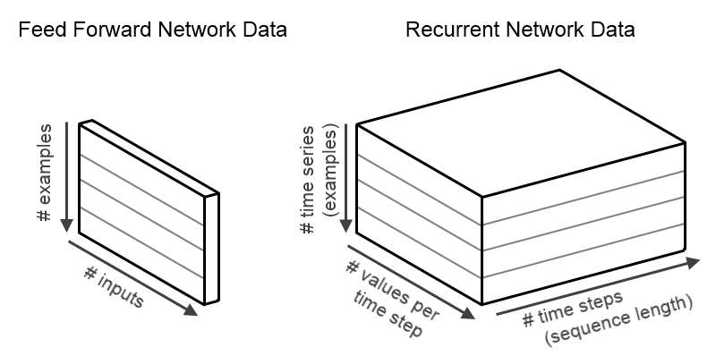
Consider for the moment a standard feed-forward network (a multi-layer perceptron or ‘DenseLayer’ in DL4J). These networks expect input and output data that is two-dimensional: that is, data with “shape” [numExamples,inputSize]. This means that the data into a feed-forward network has ‘numExamples’ rows/examples, where each row consists of ‘inputSize’ columns. A single example would have shape [1,inputSize], though in practice we generally use multiple examples for computational and optimization efficiency. Similarly, output data for a standard feed-forward network is also two dimensional, with shape [numExamples,outputSize].
Conversely, data for RNNs are time series. Thus, they have 3 dimensions: one additional dimension for time. Input data thus has shape [numExamples,inputSize,timeSeriesLength], and output data has shape [numExamples,outputSize,timeSeriesLength]. This means that the data in our INDArray is laid out such that the value at position (i,j,k) is the jth value at the kth time step of the ith example in the minibatch. This data layout is shown below.
When importing time series data using the class CSVSequenceRecordReader each line in the data files represents one time step with the earliest time series observation in the first row (or first row after header if present) and the most recent observation in the last row of the csv. Each feature time series is a separate column of the of the csv file. For example if you have five features in time series, each with 120 observations, and a training & test set of size 53 then there will be 106 input csv files(53 input, 53 labels). The 53 input csv files will each have five columns and 120 rows. The label csv files will have one column (the label) and one row.
RnnOutputLayer
RnnOutputLayer is a type of layer used as the final layer with many recurrent neural network systems (for both regression and classification tasks). RnnOutputLayer handles things like score calculation, and error calculation (of prediction vs. actual) given a loss function etc. Functionally, it is very similar to the ‘standard’ OutputLayer class (which is used with feed-forward networks); however it both outputs (and expects as labels/targets) 3d time series data sets.
Configuration for the RnnOutputLayer follows the same design other layers: for example, to set the third layer in a MultiLayerNetwork to a RnnOutputLayer for classification:
.layer(2, new RnnOutputLayer.Builder(LossFunction.MCXENT).activation(Activation.SOFTMAX)
.weightInit(WeightInit.XAVIER).nIn(prevLayerSize).nOut(nOut).build())
Use of RnnOutputLayer in practice can be seen in the examples, linked at the end of this document.
RNN Training Features
Truncated Back Propagation Through Time
Training neural networks (including RNNs) can be quite computationally demanding. For recurrent neural networks, this is especially the case when we are dealing with long sequences - i.e., training data with many time steps.
Truncated backpropagation through time (BPTT) was developed in order to reduce the computational complexity of each parameter update in a recurrent neural network. In summary, it allows us to train networks faster (by performing more frequent parameter updates), for a given amount of computational power. It is recommended to use truncated BPTT when your input sequences are long (typically, more than a few hundred time steps).
Consider what happens when training a recurrent neural network with a time series of length 12 time steps. Here, we need to do a forward pass of 12 steps, calculate the error (based on predicted vs. actual), and do a backward pass of 12 time steps:
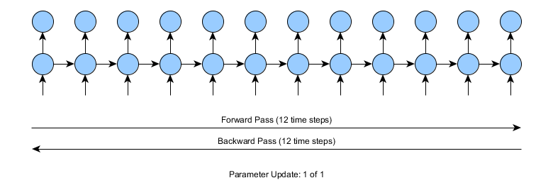
For 12 time steps, in the image above, this is not a problem. Consider, however, that instead the input time series was 10,000 or more time steps. In this case, standard backpropagation through time would require 10,000 time steps for each of the forward and backward passes for each and every parameter update. This is of course very computationally demanding.
In practice, truncated BPTT splits the forward and backward passes into a set of smaller forward/backward pass operations. The specific length of these forward/backward pass segments is a parameter set by the user. For example, if we use truncated BPTT of length 4 time steps, learning looks like the following:
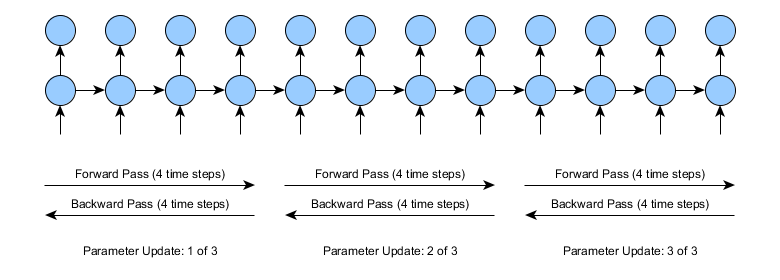
Note that the overall complexity for truncated BPTT and standard BPTT are approximately the same - both do the same number of time step during forward/backward pass. Using this method however, we get 3 parameter updates instead of one for approximately the same amount of effort. However, the cost is not exactly the same there is a small amount of overhead per parameter update.
The downside of truncated BPTT is that the length of the dependencies learned in truncated BPTT can be shorter than in full BPTT. This is easy to see: consider the images above, with a TBPTT length of 4. Suppose that at time step 10, the network needs to store some information from time step 0 in order to make an accurate prediction. In standard BPTT, this is ok: the gradients can flow backwards all the way along the unrolled network, from time 10 to time 0. In truncated BPTT, this is problematic: the gradients from time step 10 simply don’t flow back far enough to cause the required parameter updates that would store the required information. This tradeoff is usually worth it, and (as long as the truncated BPTT lengths are set appropriately), truncated BPTT works well in practice.
Using truncated BPTT in DL4J is quite simple: just add the following code to your network configuration (at the end, before the final .build() in your network configuration)
.backpropType(BackpropType.TruncatedBPTT)
.tBPTTLength(100)
The above code snippet will cause any network training (i.e., calls to MultiLayerNetwork.fit() methods) to use truncated BPTT with segments of length 100 steps.
Some things of note:
- By default (if a backprop type is not manually specified), DL4J will use BackpropType.Standard (i.e., full BPTT).
- The tBPTTLength configuration parameter set the length of the truncated BPTT passes. Typically, this is somewhere on the order of 50 to 200 time steps, though depends on the application and data.
- The truncated BPTT lengths is typically a fraction of the total time series length (i.e., 200 vs. sequence length 1000), but variable length time series in the same minibatch is OK when using TBPTT (for example, a minibatch with two sequences - one of length 100 and another of length 1000 - with a TBPTT length of 200 - will work correctly)
Masking: One-to-Many, Many-to-One, and Sequence Classification
DL4J supports a number of related training features for RNNs, based on the idea of padding and masking. Padding and masking allows us to support training situations including one-to-many, many-to-one, as also support variable length time series (in the same mini-batch).
Suppose we want to train a recurrent neural network with inputs or outputs that don’t occur at every time step. Examples of this (for a single example) are shown in the image below. DL4J supports training networks for all of these situations:

Without masking and padding, we are restricted to the many-to-many case (above, left): that is, (a) All examples are of the same length, and (b) Examples have both inputs and outputs at all time steps.
The idea behind padding is simple. Consider two time series of lengths 50 and 100 time steps, in the same mini-batch. The training data is a rectangular array; thus, we pad (i.e., add zeros to) the shorter time series (for both input and output), such that the input and output are both the same length (in this example: 100 time steps).
Of course, if this was all we did, it would cause problems during training. Thus, in addition to padding, we use a masking mechanism. The idea behind masking is simple: we have two additional arrays that record whether an input or output is actually present for a given time step and example, or whether the input/output is just padding.
Recall that with RNNs, our minibatch data has 3 dimensions, with shape [miniBatchSize,inputSize,timeSeriesLength] and [miniBatchSize,outputSize,timeSeriesLength] for the input and output respectively. The padding arrays are then 2 dimensional, with shape [miniBatchSize,timeSeriesLength] for both the input and output, with values of 0 (‘absent’) or 1 (‘present’) for each time series and example. The masking arrays for the input and output are stored in separate arrays.
For a single example, the input and output masking arrays are shown below:

For the “Masking not required” cases, we could equivalently use a masking array of all 1s, which will give the same result as not having a mask array at all. Also note that it is possible to use zero, one or two masking arrays when learning RNNs - for example, the many-to-one case could have a masking array for the output only.
In practice: these padding arrays are generally created during the data import stage (for example, by the SequenceRecordReaderDatasetIterator – discussed later), and are contained within the DataSet object. If a DataSet contains masking arrays, the MultiLayerNetwork fit will automatically use them during training. If they are absent, no masking functionality is used.
Evaluation and Scoring with Masking
Mask arrays are also important when doing scoring and evaluation (i.e., when evaluating the accuracy of a RNN classifier). Consider for example the many-to-one case: there is only a single output for each example, and any evaluation should take this into account.
Evaluation using the (output) mask arrays can be used during evaluation by passing it to the following method:
Evaluation.evalTimeSeries(INDArray labels, INDArray predicted, INDArray outputMask)
where labels are the actual output (3d time series), predicted is the network predictions (3d time series, same shape as labels), and outputMask is the 2d mask array for the output. Note that the input mask array is not required for evaluation.
Score calculation will also make use of the mask arrays, via the MultiLayerNetwork.score(DataSet) method. Again, if the DataSet contains an output masking array, it will automatically be used when calculating the score (loss function - mean squared error, negative log likelihood etc) for the network.
Masking and Sequence Classification After Training
Sequence classification is one common use of masking. The idea is that although we have a sequence (time series) as input, we only want to provide a single label for the entire sequence (rather than one label at each time step in the sequence).
However, RNNs by design output sequences, of the same length of the input sequence. For sequence classification, masking allows us to train the network with this single label at the final time step - we essentially tell the network that there isn’t actually label data anywhere except for the last time step.
Now, suppose we’ve trained our network, and want to get the last time step for predictions, from the time series output array. How do we do that?
To get the last time step, there are two cases to be aware of. First, when we have a single example, we don’t actually need to use the mask arrays: we can just get the last time step in the output array:
    INDArray timeSeriesFeatures = ...;
    INDArray timeSeriesOutput = myNetwork.output(timeSeriesFeatures);
    int timeSeriesLength = timeSeriesOutput.size(2);		//Size of time dimension
    INDArray lastTimeStepProbabilities = timeSeriesOutput.get(NDArrayIndex.point(0), NDArrayIndex.all(), NDArrayIndex.point(timeSeriesLength-1));
Assuming classification (same process for regression, however) the last line above gives us probabilities at the last time step - i.e., the class probabilities for our sequence classification.
The slightly more complex case is when we have multiple examples in the one minibatch (features array), where the lengths of each example differ. (If all are the same length: we can use the same process as above).
In this ‘variable length’ case, we need to get the last time step for each example separately. If we have the time series lengths for each example from our data pipeline, it becomes straightforward: we just iterate over examples, replacing the timeSeriesLength in the above code with the length of that example.
If we don’t have the lengths of the time series directly, we need to extract them from the mask array.
If we have a labels mask array (which is a one-hot vector, like [0,0,0,1,0] for each time series):
    INDArray labelsMaskArray = ...;
    INDArray lastTimeStepIndices = Nd4j.argMax(labelMaskArray,1);
Alternatively, if we have only the features mask: One quick and dirty approach is to use this:
    INDArray featuresMaskArray = ...;
    int longestTimeSeries = featuresMaskArray.size(1);
    INDArray linspace = Nd4j.linspace(1,longestTimeSeries,longestTimeSeries);
    INDArray temp = featuresMaskArray.mulColumnVector(linspace);
    INDArray lastTimeStepIndices = Nd4j.argMax(temp,1);
To understand what is happening here, note that originally we have a features mask like [1,1,1,1,0], from which we want to get the last non-zero element. So we map [1,1,1,1,0] -> [1,2,3,4,0], and then get the largest element (which is the last time step).
In either case, we can then do the following:
    int numExamples = timeSeriesFeatures.size(0);
    for( int i=0; i<numExamples; i++ ){
        int thisTimeSeriesLastIndex = lastTimeStepIndices.getInt(i);
        INDArray thisExampleProbabilities = timeSeriesOutput.get(NDArrayIndex.point(i), NDArrayIndex.all(), NDArrayIndex.point(thisTimeSeriesLastIndex));
    }
Combining RNN Layers with Other Layer Types
RNN layers in DL4J can be combined with other layer types. For example, it is possible to combine DenseLayer and GravesLSTM layers in the same network; or combine Convolutional (CNN) layers and GravesLSTM layers for video.
Of course, the DenseLayer and Convolutional layers do not handle time series data - they expect a different type of input. To deal with this, we need to use the layer preprocessor functionality: for example, the CnnToRnnPreProcessor and FeedForwardToRnnPreprocessor classes. See here for all preprocessors. Fortunately, in most situations, the DL4J configuration system will automatically add these preprocessors as required. However, the preprocessors can be added manually (overriding the automatic addition of preprocessors, for each layer).
For example, to manually add a preprocessor between layers 1 and 2, add the following to your network configuration: .inputPreProcessor(2, new RnnToFeedForwardPreProcessor()).
Test Time: Predictions One Step at a Time
As with other types of neural networks, predictions can be generated for RNNs using the MultiLayerNetwork.output() and MultiLayerNetwork.feedForward() methods. These methods can be useful in many circumstances; however, they have the limitation that we can only generate predictions for time series, starting from scratch each and every time.
Consider for example the case where we want to generate predictions in a real-time system, where these predictions are based on a very large amount of history. It this case, it is impractical to use the output/feedForward methods, as they conduct the full forward pass over the entire data history, each time they are called. If we wish to make a prediction for a single time step, at every time step, these methods can be both (a) very costly, and (b) wasteful, as they do the same calculations over and over.
For these situations, MultiLayerNetwork provides four methods of note:
rnnTimeStep(INDArray)rnnClearPreviousState()rnnGetPreviousState(int layer)rnnSetPreviousState(int layer, Map<String,INDArray> state)
The rnnTimeStep() method is designed to allow forward pass (predictions) to be conducted efficiently, one or more steps at a time. Unlike the output/feedForward methods, the rnnTimeStep method keeps track of the internal state of the RNN layers when it is called. It is important to note that output for the rnnTimeStep and the output/feedForward methods should be identical (for each time step), whether we make these predictions all at once (output/feedForward) or whether these predictions are generated one or more steps at a time (rnnTimeStep). Thus, the only difference should be the computational cost.
In summary, the MultiLayerNetwork.rnnTimeStep() method does two things:
- Generate output/predictions (forward pass), using the previous stored state (if any)
- Update the stored state, storing the activations for the last time step (ready to be used next time rnnTimeStep is called)
For example, suppose we want to use a RNN to predict the weather, one hour in advance (based on the weather at say the previous 100 hours as input). If we were to use the output method, at each hour we would need to feed in the full 100 hours of data to predict the weather for hour 101. Then to predict the weather for hour 102, we would need to feed in the full 100 (or 101) hours of data; and so on for hours 103+.
Alternatively, we could use the rnnTimeStep method. Of course, if we want to use the full 100 hours of history before we make our first prediction, we still need to do the full forward pass:

For the first time we call rnnTimeStep, the only practical difference between the two approaches is that the activations/state of the last time step are stored - this is shown in orange. However, the next time we use the rnnTimeStep method, this stored state will be used to make the next predictions:
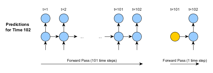
There are a number of important differences here:
- In the second image (second call of rnnTimeStep) the input data consists of a single time step, instead of the full history of data
- The forward pass is thus a single time step (as compared to the hundreds – or more)
- After the rnnTimeStep method returns, the internal state will automatically be updated. Thus, predictions for time 103 could be made in the same way as for time 102. And so on.
However, if you want to start making predictions for a new (entirely separate) time series: it is necessary (and important) to manually clear the stored state, using the MultiLayerNetwork.rnnClearPreviousState() method. This will reset the internal state of all recurrent layers in the network.
If you need to store or set the internal state of the RNN for use in predictions, you can use the rnnGetPreviousState and rnnSetPreviousState methods, for each layer individually. This can be useful for example during serialization (network saving/loading), as the internal network state from the rnnTimeStep method is not saved by default, and must be saved and loaded separately. Note that these get/set state methods return and accept a map, keyed by the type of activation. For example, in the LSTM model, it is necessary to store both the output activations, and the memory cell state.
Some other points of note:
- We can use the rnnTimeStep method for multiple independent examples/predictions simultaneously. In the weather example above, we might for example want to make predicts for multiple locations using the same neural network. This works in the same way as training and the forward pass / output methods: multiple rows (dimension 0 in the input data) are used for multiple examples.
- If no history/stored state is set (i.e., initially, or after a call to rnnClearPreviousState), a default initialization (zeros) is used. This is the same approach as during training.
- The rnnTimeStep can be used for an arbitrary number of time steps simultaneously – not just one time step. However, it is important to note:
- For a single time step prediction: the data is 2 dimensional, with shape [numExamples,nIn]; in this case, the output is also 2 dimensional, with shape [numExamples,nOut]
- For multiple time step predictions: the data is 3 dimensional, with shape [numExamples,nIn,numTimeSteps]; the output will have shape [numExamples,nOut,numTimeSteps]. Again, the final time step activations are stored as before.
- It is not possible to change the number of examples between calls of rnnTimeStep (in other words, if the first use of rnnTimeStep is for say 3 examples, all subsequent calls must be with 3 examples). After resetting the internal state (using rnnClearPreviousState()), any number of examples can be used for the next call of rnnTimeStep.
- The rnnTimeStep method makes no changes to the parameters; it is used after training the network has been completed only.
- The rnnTimeStep method works with networks containing single and stacked/multiple RNN layers, as well as with networks that combine other layer types (such as Convolutional or Dense layers).
- The RnnOutputLayer layer type does not have any internal state, as it does not have any recurrent connections.
Importing Time Series Data
Data import for RNNs is complicated by the fact that we have multiple different types of data we could want to use for RNNs: one-to-many, many-to-one, variable length time series, etc. This section will describe the currently implemented data import mechanisms for DL4J.
The methods described here utilize the SequenceRecordReaderDataSetIterator class, in conjunction with the CSVSequenceRecordReader class from DataVec. This approach currently allows you to load delimited (tab, comma, etc) data from files, where each time series is in a separate file. This method also supports:
- Variable length time series input
- One-to-many and many-to-one data loading (where input and labels are in different files)
- Label conversion from an index to a one-hot representation for classification (i.e., ‘2’ to [0,0,1,0])
- Skipping a fixed/specified number of rows at the start of the data files (i.e., comment or header rows)
Note that in all cases, each line in the data files represents one time step.
(In addition to the examples below, you might find these unit tests to be of some use.)
Example 1: Time Series of Same Length, Input and Labels in Separate Files
Suppose we have 10 time series in our training data, represented by 20 files: 10 files for the input of each time series, and 10 files for the output/labels. For now, assume these 20 files all contain the same number of time steps (i.e., same number of rows).
To use the SequenceRecordReaderDataSetIterator and CSVSequenceRecordReader approaches, we first create two CSVSequenceRecordReader objects, one for input and one for labels:
SequenceRecordReader featureReader = new CSVSequenceRecordReader(1, ",");
SequenceRecordReader labelReader = new CSVSequenceRecordReader(1, ",");
This particular constructor takes the number of lines to skip (1 row skipped here), and the delimiter (comma character used here).
Second, we need to initialize these two readers, by telling them where to get the data from. We do this with an InputSplit object. Suppose that our time series are numbered, with file names “myInput_0.csv”, “myInput_1.csv”, …, “myLabels_0.csv”, etc. One approach is to use the NumberedFileInputSplit:
featureReader.initialize(new NumberedFileInputSplit("/path/to/data/myInput_%d.csv", 0, 9));
labelReader.initialize(new NumberedFileInputSplit(/path/to/data/myLabels_%d.csv", 0, 9));
In this particular approach, the “%d” is replaced by the corresponding number, and the numbers 0 to 9 (both inclusive) are used.
Finally, we can create our SequenceRecordReaderdataSetIterator:
DataSetIterator iter = new SequenceRecordReaderDataSetIterator(featureReader, labelReader, miniBatchSize, numPossibleLabels, regression);
This DataSetIterator can then be passed to MultiLayerNetwork.fit() to train the network.
The miniBatchSize argument specifies the number of examples (time series) in each minibatch. For example, with 10 files total, miniBatchSize of 5 would give us two data sets with 2 minibatches (DataSet objects) with 5 time series in each.
Note that:
- For classification problems: numPossibleLabels is the number of classes in your data set. Use regression = false.
- Labels data: one value per line, as a class index
- Label data will be converted to a one-hot representation automatically
- For regression problems: numPossibleLabels is not used (set it to anything) and use regression = true.
- The number of values in the input and labels can be anything (unlike classification: can have an arbitrary number of outputs)
- No processing of the labels is done when regression = true
Example 2: Time Series of Same Length, Input and Labels in Same File
Following on from the last example, suppose that instead of a separate files for our input data and labels, we have both in the same file. However, each time series is still in a separate file.
As of DL4J 0.4-rc3.8, this approach has the restriction of a single column for the output (either a class index, or a single real-valued regression output)
In this case, we create and initialize a single reader. Again, we are skipping one header row, and specifying the format as comma delimited, and assuming our data files are named “myData_0.csv”, …, “myData_9.csv”:
SequenceRecordReader reader = new CSVSequenceRecordReader(1, ",");
reader.initialize(new NumberedFileInputSplit("/path/to/data/myData_%d.csv", 0, 9));
DataSetIterator iterClassification = new SequenceRecordReaderDataSetIterator(reader, miniBatchSize, numPossibleLabels, labelIndex, false);
miniBatchSize and numPossibleLabels are the same as the previous example. Here, labelIndex specifies which column the labels are in. For example, if the labels are in the fifth column, use labelIndex = 4 (i.e., columns are indexed 0 to numColumns-1).
For regression on a single output value, we use:
DataSetIterator iterRegression = new SequenceRecordReaderDataSetIterator(reader, miniBatchSize, -1, labelIndex, true);
Again, the numPossibleLabels argument is not used for regression.
Example 3: Time Series of Different Lengths (Many-to-Many)
Following on from the previous two examples, suppose that for each example individually, the input and labels are of the same length, but these lengths differ between time series.
We can use the same approach (CSVSequenceRecordReader and SequenceRecordReaderDataSetIterator), though with a different constructor:
DataSetIterator variableLengthIter = new SequenceRecordReaderDataSetIterator(featureReader, labelReader, miniBatchSize, numPossibleLabels, regression, SequenceRecordReaderDataSetIterator.AlignmentMode.ALIGN_END);
The argument here are the same as in the previous example, with the exception of the AlignmentMode.ALIGN_END addition. This alignment mode input tells the SequenceRecordReaderDataSetIterator to expect two things:
- That the time series may be of different lengths
- To align the input and labels - for each example individually - such that their last values occur at the same time step.
Note that if the features and labels are always of the same length (as is the assumption in example 3), then the two alignment modes (AlignmentMode.ALIGN_END and AlignmentMode.ALIGN_START) will give identical outputs. The alignment mode option is explained in the next section.
Also note: that variable length time series always start at time zero in the data arrays: padding, if required, will be added after the time series has ended.
Unlike examples 1 and 2 above, the DataSet objects produced by the above variableLengthIter instance will also include input and masking arrays, as described earlier in this document.
Example 4: Many-to-One and One-to-Many Data
We can also use the AlignmentMode functionality in example 3 to implement a many-to-one RNN sequence classifier. Here, let us assume:
- Input and labels are in separate delimited files
- The labels files contain a single row (time step) (either a class index for classification, or one or more numbers for regression)
- The input lengths may (optionally) differ between examples
In fact, the same approach as in example 3 can do this:
DataSetIterator variableLengthIter = new SequenceRecordReaderDataSetIterator(featureReader, labelReader, miniBatchSize, numPossibleLabels, regression, SequenceRecordReaderDataSetIterator.AlignmentMode.ALIGN_END);
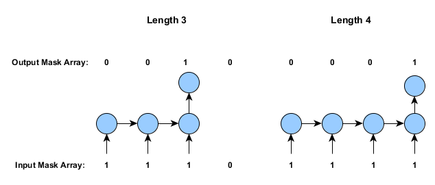
Alignment modes are relatively straightforward. They specify whether to pad the start or the end of the shorter time series. The diagram below shows how this works, along with the masking arrays (as discussed earlier in this document):

The one-to-many case (similar to the last case above, but with only one input) is done by using AlignmentMode.ALIGN_START.
Note that in the case of training data that contains time series of different lengths, the labels and inputs will be aligned for each example individually, and then the shorter time series will be padded as required:
Alternative: Implementing a custom DataSetIterator
In some cases, you will have to do something that doesn’t fit into a typical data import scenario. One option for this scenario is to implement a custom DataSetIterator. DataSetIterator is merely an interface for iterating over DataSet objects - objects that encapsulate the input and target INDArrays, plus (optionally) the input and labels mask arrays.
Note however that this approach is quite low level: implementing a DataSetIterator requires you to manually create the required INDArrays for the input and the labels, as well as (if required) the input and labels mask arrays. However, this approach gives you a great degree of flexibility over exactly how data is loaded.
For example of this approach in practice, see the the iterator for the character example and for the Word2Vec movie review sentiment example.
Note: When creating a custom DataSetIterator, it is important that your data arrays - the input features, the labels, and any mask arrays - are created in ‘f’ (fortran) order. See the ND4J user guide for details on array orders. In practice, this means using the Nd4j.create methods that allow you to specify the array order: Nd4j.create(new int[]{numExamples, inputSize, timeSeriesLength},'f'). Though ‘c’ order arrays will also work, performance will be reduced due to the need to copy the arrays to ‘f’ order first, for certain operations.
Examples
DL4J currently has the following recurrent neural network examples:
- A character modelling example, which generates Shakespearean prose, one character at a time
- A basic video frame classification example, that imports videos (.mp4 format) and classifies the shapes present in each frame
- A word2vec sequence classification example that uses pre-trained word vectors and a RNN to classify movie reviews as either positive or negative.